Loss Functions: Measuring Model Performance
Introduction
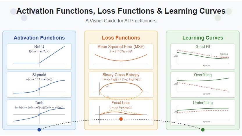
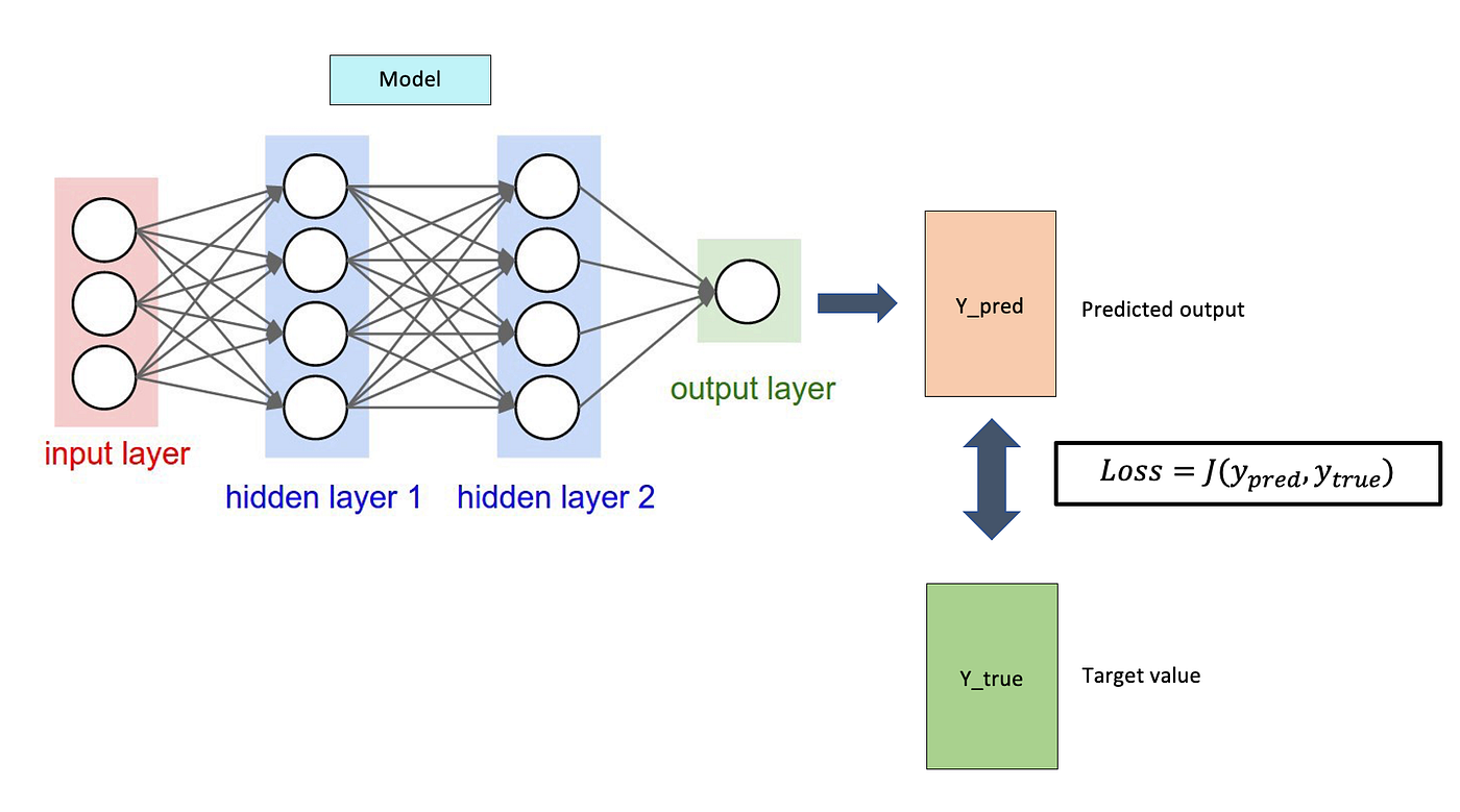
Loss functions are the compass that guides neural networks during training. They quantify how far your model's predictions are from the true values, providing a single numerical score that optimization algorithms use to improve the model. The choice of loss function can make or break your model's performance—use the wrong one, and your model might never converge or learn the wrong patterns entirely.
Every training iteration follows the same pattern: forward pass → compute loss → backward pass → update weights. The loss function sits at the heart of this cycle, translating the gap between predictions and reality into gradients that drive learning.
graph LR
    A[Input Data] --> B[Forward Pass]
    B --> C[Model Predictions]
    C --> D[Compute Loss]
    E[True Labels] --> D
    D --> F[Backward Pass]
    F --> G[Compute Gradients]
    G --> H[Update Weights]
    H --> B
    style D fill:#ff6b6b,stroke:#c92a2a,stroke-width:3px,color:#fff
In this article, we'll explore the most commonly used loss functions, their mathematical foundations, when to use each one, and how to avoid common pitfalls that can derail training.
What is a Loss Function?
A loss function (also called a cost function or objective function) is a mathematical function that measures the discrepancy between predicted values ($\hat{y}$) and true values ($y$). It outputs a single scalar value that represents how well (or poorly) your model is performing.
Mathematical Definition:
$$ \mathcal{L} = f(\hat{y}, y) $$
Where:
- $\mathcal{L}$ is the loss value
- $\hat{y}$ are the model's predictions
- $y$ are the true target values
- $f$ is the loss function
The Training Objective: Minimize the loss function
$$ \theta^* = \arg\min_{\theta} \mathcal{L}(f_\theta(x), y) $$
Where $\theta$ represents the model's parameters (weights and biases).
Reduction Methods
Most loss functions compute a loss value for each sample in a batch. PyTorch provides three ways to aggregate these individual losses:
| Reduction | Formula | Use Case |
|---|---|---|
| mean (default) | $\mathcal{L} = \frac{1}{N}\sum_{i=1}^{N} \ell_i$ | Most common; provides stable gradients |
| sum | $\mathcal{L} = \sum_{i=1}^{N} \ell_i$ | When you want absolute loss magnitude; rare |
| none | $\mathcal{L} = [\ell_1, \ell_2, ..., \ell_N]$ | For custom aggregation or per-sample analysis |
import torch.nn as nn

# Different reduction modes
criterion_mean = nn.MSELoss(reduction='mean')   # Default
criterion_sum = nn.MSELoss(reduction='sum')
criterion_none = nn.MSELoss(reduction='none')   # Returns loss per sample
Regression Losses: For continuous predictions (e.g., prices). Classification Losses: For discrete labels (e.g., spam/not spam).
Regression Loss Functions
Regression tasks involve predicting continuous values (house prices, temperature, stock prices). The choice of loss function determines how the model penalizes prediction errors.
graph LR
    A[Regression Tasks] --> B[MSE]
    A --> C[MAE]
    A --> D[Smooth L1]
    B --> E[Quadratic Penalty<br/>Sensitive to outliers]
    C --> F[Linear Penalty<br/>Robust to outliers]
    D --> G[Hybrid Approach<br/>Best of both]
    style B fill:#fa5252,stroke:#c92a2a
    style C fill:#51cf66,stroke:#2f9e44
    style D fill:#ffd43b,stroke:#f59f00
1. Mean Squared Error (MSE) / L2 Loss
Mathematical Formula:
$$ \text{MSE} = \frac{1}{N}\sum_{i=1}^{N}(y_i - \hat{y}_i)^2 $$
Derivative:
$$ \frac{\partial L}{\partial \hat{y}_i} = \frac{2}{N}(\hat{y}_i - y_i) $$
Key Characteristics:
- Quadratic penalty: Errors are squared, so large errors are penalized exponentially more than small ones
- Differentiable everywhere: Smooth gradients throughout
- Scale-dependent: Sensitive to the scale of the target variable
Advantages:
- Most commonly used regression loss
- Unique optimal solution (convex for linear models)
- Penalizes large errors heavily, encouraging accurate predictions
- Well-understood mathematical properties
- Differentiable everywhere
Disadvantages:
- Very sensitive to outliers: A single outlier can dominate the loss
- Can lead to exploding gradients if predictions are far from targets
- Not robust to noisy data
- Assumes errors are normally distributed
Best Use Cases:
- Clean datasets without outliers
- When large errors are significantly worse than small errors
- Default choice for most regression problems
- When you want to minimize variance in predictions
PyTorch Implementation:
import torch
import torch.nn as nn

# Basic usage
predictions = torch.tensor([2.5, 3.0, 4.5])
targets = torch.tensor([2.0, 3.5, 4.0])

mse_loss = nn.MSELoss()
loss = mse_loss(predictions, targets)
print(f"MSE Loss: {loss.item():.4f}")
# Output: MSE Loss: 0.1667
Practical Example:
import torch
import torch.nn as nn

class RegressionModel(nn.Module):
    def __init__(self, input_size):
        super().__init__()
        self.model = nn.Sequential(
            nn.Linear(input_size, 64),
            nn.ReLU(),
            nn.Linear(64, 32),
            nn.ReLU(),
            nn.Linear(32, 1)  # Single output for regression
        )

    def forward(self, x):
        return self.model(x)

# Training setup
model = RegressionModel(input_size=10)
criterion = nn.MSELoss()
optimizer = torch.optim.Adam(model.parameters(), lr=0.001)

# Training loop
for epoch in range(100):
    predictions = model(X_train)
    loss = criterion(predictions, y_train)

    optimizer.zero_grad()
    loss.backward()
    optimizer.step()
2. Mean Absolute Error (MAE) / L1 Loss
Mathematical Formula:
$$ \text{MAE} = \frac{1}{N}\sum_{i=1}^{N}|y_i - \hat{y}_i| $$
Derivative:
$$ \frac{\partial L}{\partial \hat{y}_i} = \frac{1}{N} \cdot \text{sgn}(\hat{y}_i - y_i) $$
Key Characteristics:
- Linear penalty: All errors weighted equally regardless of magnitude
- Robust to outliers: Outliers don't dominate the loss
- Constant gradient: Gradient magnitude is the same for all errors
Advantages:
- Robust to outliers: Outliers have linear (not quadratic) impact
- More interpretable: Loss value is in the same units as target variable
- Stable gradients (constant magnitude)
- Better for data with many outliers or heavy-tailed distributions
Disadvantages:
- Gradient is constant, which can lead to instability near convergence (large updates even when close to optimum)
- Not differentiable at zero (but subgradient works in practice)
- May converge slower than MSE for clean data
- Can oscillate around the minimum without proper learning rate decay
Best Use Cases:
- Datasets with outliers or noisy labels
- When all errors should be weighted equally
- Predicting medians rather than means
- Robust regression tasks
PyTorch Implementation:
import torch
import torch.nn as nn

predictions = torch.tensor([2.5, 3.0, 10.0])  # 10.0 is an outlier
targets = torch.tensor([2.0, 3.5, 4.0])

# MSE is heavily affected by the outlier
mse_loss = nn.MSELoss()
print(f"MSE Loss: {mse_loss(predictions, targets).item():.4f}")
# Output: MSE Loss: 12.1667 (dominated by outlier)

# MAE is more robust
mae_loss = nn.L1Loss()
print(f"MAE Loss: {mae_loss(predictions, targets).item():.4f}")
# Output: MAE Loss: 2.1667 (less affected by outlier)
Comparison: MSE vs MAE with Outliers
import torch
import matplotlib.pyplot as plt

# Predictions with one outlier
predictions = torch.tensor([2.1, 3.0, 2.9, 3.2, 15.0])  # 15.0 is outlier
targets = torch.tensor([2.0, 3.0, 3.0, 3.0, 3.0])

mse = nn.MSELoss()(predictions, targets)
mae = nn.L1Loss()(predictions, targets)

print(f"MSE: {mse:.2f} (heavily penalizes outlier)")
print(f"MAE: {mae:.2f} (more robust to outlier)")
# MSE: 28.88
# MAE: 2.44

3. Smooth L1 Loss (Huber Loss)
Mathematical Formula:
$$
\text{SmoothL1}(x) = \begin{cases}
0.5x^2 & |x| < \beta \
\beta(|x| - 0.5\beta) & |x| \geq \beta
\end{cases}
$$
Where $x = \hat{y} - y$ and $\beta$ is a threshold (default: 1.0 in PyTorch)
Key Characteristics:
- Hybrid approach: Combines MSE (small errors) and MAE (large errors)
- Smooth transition: Differentiable everywhere
- Less sensitive to outliers than MSE but converges faster than MAE
Advantages:
- Best of both worlds: Fast convergence + outlier robustness
- Smooth gradients (unlike MAE at zero)
- Less sensitive to outliers than MSE
- Controlled gradient magnitude for large errors
- Used successfully in object detection (Faster R-CNN)
Disadvantages:
- Requires tuning $\beta$ hyperparameter
- More complex than MSE or MAE
- Less interpretable
- Slightly more computational overhead
Best Use Cases:
- Object detection (bounding box regression)
- When you expect some outliers but want faster convergence than MAE
- Tasks requiring both precision (small errors) and robustness (large errors)
- Default choice for many computer vision regression tasks
PyTorch Implementation:
import torch
import torch.nn as nn

predictions = torch.tensor([2.5, 3.0, 10.0])
targets = torch.tensor([2.0, 3.5, 4.0])

smooth_l1 = nn.SmoothL1Loss(beta=1.0)
loss = smooth_l1(predictions, targets)
print(f"Smooth L1 Loss: {loss.item():.4f}")

# Compare with MSE and MAE
print(f"MSE Loss: {nn.MSELoss()(predictions, targets).item():.4f}")
print(f"MAE Loss: {nn.L1Loss()(predictions, targets).item():.4f}")
Visualizing the Difference:
import torch
import matplotlib.pyplot as plt

errors = torch.linspace(-3, 3, 100)

# MSE: Quadratic everywhere
mse = 0.5 * errors ** 2

# MAE: Linear everywhere
mae = torch.abs(errors)

# Smooth L1: Quadratic near zero, linear for large errors
smooth_l1 = torch.where(
    torch.abs(errors) < 1,
    0.5 * errors ** 2,
    torch.abs(errors) - 0.5
)

# The smooth L1 curve combines the best of both

Classification Loss Functions
Classification tasks involve predicting discrete categories. The loss function must handle probability distributions and class labels effectively.
4. Binary Cross-Entropy with Logits (BCEWithLogitsLoss)
Mathematical Formula:
$$ \text{BCEWithLogits} = -\frac{1}{N}\sum_{i=1}^{N}[y_i \log(\sigma(z_i)) + (1-y_i)\log(1-\sigma(z_i))] $$
Where:
- $\sigma(z) = \frac{1}{1+e^{-z}}$ is the sigmoid function
- $z$ are raw logits (model outputs)
- $y_i \in {0, 1}$ are true labels
Key Characteristics:
This loss combines sigmoid and binary cross-entropy in a single numerically stable operation:
- Numerical stability: Uses log-sum-exp trick to avoid overflow/underflow
- Better gradients: Prevents gradient saturation
- Simpler architecture: No sigmoid needed in model
Advantages:
- Numerically stable: Uses log-sum-exp trick internally
- More stable gradients during training
- No need for sigmoid in model (cleaner architecture)
- Recommended over plain BCE in almost all cases
- Can handle pos_weight for class imbalance
Best Use Cases:
- Binary classification (2 classes)
- Multi-label classification (multiple independent binary predictions)
- When dealing with class imbalance (use
pos_weightparameter) - Default choice for any binary classification task
PyTorch Implementation:
import torch
import torch.nn as nn

# Raw logits (NO sigmoid in model!)
logits = torch.tensor([[2.3], [-1.5], [3.0]])  # Raw model outputs
targets = torch.tensor([[1.0], [0.0], [1.0]])

bce_with_logits = nn.BCEWithLogitsLoss()
loss = bce_with_logits(logits, targets)
print(f"BCE with Logits: {loss.item():.4f}")

# Recommended model structure
class BinaryClassifierCorrect(nn.Module):
    def __init__(self, input_size):
        super().__init__()
        self.model = nn.Sequential(
            nn.Linear(input_size, 64),
            nn.ReLU(),
            nn.Linear(64, 1)
            # NO sigmoid here!
        )

    def forward(self, x):
        return self.model(x)

# Use with BCEWithLogitsLoss
model = BinaryClassifierCorrect(10)
criterion = nn.BCEWithLogitsLoss()
Handling Class Imbalance:
# If positive class is rare (e.g., 1:10 ratio)
# Increase weight for positive class
pos_weight = torch.tensor([10.0])  # 10x weight for positive class
criterion = nn.BCEWithLogitsLoss(pos_weight=pos_weight)
5. Cross-Entropy Loss
Mathematical Formula:
For multi-class classification with $C$ classes:
$$ \text{CrossEntropy} = -\sum_{i=1}^{N} \log\left(\frac{e^{z_{y_i}}}{\sum_{j=1}^{C} e^{z_j}}\right) $$
Where:
- $z$ are raw logits (model outputs)
- $y_i$ is the true class index
- The formula includes softmax internally
Expanded Form:
$$ \text{CrossEntropy} = -\sum_{i=1}^{N} \sum_{c=1}^{C} y_{i,c} \log(\hat{y}_{i,c}) $$
Where $y_{i,c}$ is 1 if sample $i$ belongs to class $c$, else 0.
Key Characteristics:
- Combines softmax and negative log-likelihood
- Expects raw logits (no softmax in model!)
- Target can be class indices or probabilities
Advantages:
- Most common multi-class classification loss
- Numerically stable (log-sum-exp trick)
- Probabilistic interpretation
- Works well for most classification tasks
- Supports class weights for imbalance
Disadvantages:
- Assumes classes are mutually exclusive
- Can struggle with severe class imbalance
- Treats all misclassifications equally
- May not be ideal for hierarchical classification
Best Use Cases:
- Multi-class classification (>2 classes)
- Image classification
- Text classification
- Any task with mutually exclusive classes
PyTorch Implementation:
import torch
import torch.nn as nn

# Raw logits for 3 classes (NO softmax in model!)
logits = torch.tensor([
    [2.0, 1.0, 0.1],  # Sample 1
    [0.5, 2.5, 1.0],  # Sample 2
    [1.0, 0.5, 3.0]   # Sample 3
])

# Targets are class indices
targets = torch.tensor([0, 1, 2])  # Ground truth classes

ce_loss = nn.CrossEntropyLoss()
loss = ce_loss(logits, targets)
print(f"Cross-Entropy Loss: {loss.item():.4f}")

# Complete model example
class MultiClassClassifier(nn.Module):
    def __init__(self, input_size, num_classes):
        super().__init__()
        self.model = nn.Sequential(
            nn.Linear(input_size, 128),
            nn.ReLU(),
            nn.Dropout(0.3),
            nn.Linear(128, 64),
            nn.ReLU(),
            nn.Linear(64, num_classes)
            # NO softmax here! CrossEntropyLoss applies it internally
        )

    def forward(self, x):
        return self.model(x)

# Training
model = MultiClassClassifier(input_size=20, num_classes=10)
criterion = nn.CrossEntropyLoss()
optimizer = torch.optim.Adam(model.parameters())

# Forward pass
outputs = model(X_batch)  # Raw logits
loss = criterion(outputs, y_batch)  # Targets are class indices
Handling Class Imbalance:
# If classes are imbalanced [100, 50, 10 samples]
# Compute class weights inversely proportional to frequency
class_counts = torch.tensor([100, 50, 10])
class_weights = 1.0 / class_counts
class_weights = class_weights / class_weights.sum()  # Normalize

criterion = nn.CrossEntropyLoss(weight=class_weights)
6. Focal Loss
Mathematical Formula:
$$ \text{FocalLoss} = -\alpha_t (1 - p_t)^\gamma \log(p_t) $$
Where:
- $p_t$ is the model's estimated probability for the true class
- $\gamma$ is the focusing parameter ($\gamma \geq 0$)
- $\alpha_t$ is a weighting factor (optional)
Key Characteristics:
- Down-weights easy examples
- Focuses training on hard, misclassified examples
- $\gamma$ controls how much to down-weight easy examples
Advantages:
- Excellent for severe class imbalance (e.g., object detection)
- Focuses on hard-to-classify examples
- Reduces impact of easy negatives
- Used successfully in RetinaNet, YOLO variants
Disadvantages:
- Requires tuning $\gamma$ and $\alpha$ hyperparameters
- More complex than standard cross-entropy
- Can be sensitive to hyperparameter choices
- Not built into PyTorch (need custom implementation)
Best Use Cases:
- Severe class imbalance (1:1000+ ratios)
- Object detection
- When one class dominates the dataset
- Medical imaging (rare disease detection)
PyTorch Implementation:
import torch
import torch.nn as nn
import torch.nn.functional as F

class FocalLoss(nn.Module):
    def __init__(self, alpha=0.25, gamma=2.0, reduction='mean'):
        super().__init__()
        self.alpha = alpha
        self.gamma = gamma
        self.reduction = reduction

    def forward(self, inputs, targets):
        """
        inputs: logits (raw model outputs)
        targets: class indices
        """
        ce_loss = F.cross_entropy(inputs, targets, reduction='none')
        p_t = torch.exp(-ce_loss)  # Probability of true class
        focal_loss = self.alpha * (1 - p_t) ** self.gamma * ce_loss

        if self.reduction == 'mean':
            return focal_loss.mean()
        elif self.reduction == 'sum':
            return focal_loss.sum()
        else:
            return focal_loss

# Usage
model = MultiClassClassifier(input_size=20, num_classes=10)
criterion = FocalLoss(alpha=0.25, gamma=2.0)

outputs = model(X_batch)
loss = criterion(outputs, y_batch)
Comparison: Cross-Entropy vs Focal Loss:
# Easy example (high confidence, correct prediction)
easy_logits = torch.tensor([[5.0, 0.1, 0.1]])  # Very confident in class 0
easy_target = torch.tensor([0])

ce_easy = F.cross_entropy(easy_logits, easy_target)
focal_easy = FocalLoss()(easy_logits, easy_target)

# Hard example (low confidence, correct prediction)
hard_logits = torch.tensor([[0.6, 0.5, 0.4]])  # Uncertain
hard_target = torch.tensor([0])

ce_hard = F.cross_entropy(hard_logits, hard_target)
focal_hard = FocalLoss()(hard_logits, hard_target)

print("Easy Example:")
print(f"  CE Loss: {ce_easy:.4f}, Focal Loss: {focal_easy:.4f}")
print("Hard Example:")
print(f"  CE Loss: {ce_hard:.4f}, Focal Loss: {focal_hard:.4f}")

# Focal loss down-weights easy examples, focuses on hard ones
Loss Function Comparison Table
| Loss Function | Task Type | Input Type | Key Feature | Best For |
|---|---|---|---|---|
| MSE | Regression | Continuous values | Penalizes large errors heavily | Clean data, no outliers |
| MAE | Regression | Continuous values | Robust to outliers | Noisy data, outliers present |
| Smooth L1 | Regression | Continuous values | Hybrid MSE+MAE | Object detection, robust regression |
| BCEWithLogits | Binary Classification | Logits (raw) | Numerically stable | Binary/multi-label classification |
| CrossEntropy | Multi-class | Logits (raw) | Combines softmax+NLL | Image/text classification |
| Focal Loss | Classification (imbalanced) | Logits (raw) | Focuses on hard examples | Severe class imbalance |
Choosing the Right Loss Function
Decision Tree
graph TD
    A[What's your task?] --> B{Classification or Regression?}
    B -->|Regression| C{Data quality?}
    C -->|Clean, no outliers| D[MSE Loss]
    C -->|Has outliers| E[MAE or Smooth L1]
    C -->|Object detection| F[Smooth L1 Loss]

    B -->|Classification| G{How many classes?}
    G -->|Binary 2 classes| H{Class balance?}
    H -->|Balanced| I[BCEWithLogitsLoss]
    H -->|Imbalanced| J[BCEWithLogitsLoss<br/>+ pos_weight]

    G -->|Multi-class >2| K{Class balance?}
    K -->|Balanced| L[CrossEntropyLoss]
    K -->|Moderate imbalance| M[CrossEntropyLoss<br/>+ class weights]
    K -->|Severe imbalance<br/>1:100+| N[Focal Loss]

    style D fill:#4dabf7,stroke:#1971c2,stroke-width:2px
    style E fill:#4dabf7,stroke:#1971c2,stroke-width:2px
    style F fill:#4dabf7,stroke:#1971c2,stroke-width:2px
    style I fill:#51cf66,stroke:#2f9e44,stroke-width:2px
    style J fill:#51cf66,stroke:#2f9e44,stroke-width:2px
    style L fill:#51cf66,stroke:#2f9e44,stroke-width:2px
    style M fill:#51cf66,stroke:#2f9e44,stroke-width:2px
    style N fill:#ffd43b,stroke:#f59f00,stroke-width:2px
Quick Reference Guide
| Scenario | Recommended Loss | Alternative |
|---|---|---|
| Regression, clean data | MSE | Smooth L1 |
| Regression, outliers present | MAE | Huber Loss |
| Binary classification | BCEWithLogitsLoss | Focal Loss (imbalanced) |
| Multi-class classification | CrossEntropyLoss | Focal Loss (imbalanced) |
| Multi-label classification | BCEWithLogitsLoss | Focal Loss |
| Severe class imbalance (1:100+) | Focal Loss | Weighted CrossEntropy |
| Object detection | Smooth L1 (bbox), Focal (class) | - |
| Metric learning | Triplet Loss | Contrastive Loss |
Common Mistakes and How to Avoid Them
Mistake 1: Using Sigmoid + CrossEntropyLoss
# ❌ WRONG: CrossEntropyLoss applies softmax internally
class WrongModel(nn.Module):
    def forward(self, x):
        x = self.layers(x)
        return F.softmax(x, dim=1)  # DON'T DO THIS

criterion = nn.CrossEntropyLoss()

# ✅ CORRECT: Return raw logits
class CorrectModel(nn.Module):
    def forward(self, x):
        return self.layers(x)  # Raw logits

criterion = nn.CrossEntropyLoss()  # Applies softmax internally
Mistake 2: Wrong Target Format
# ❌ WRONG: CrossEntropyLoss expects class indices, not one-hot
targets = torch.tensor([[1, 0, 0], [0, 1, 0]])  # One-hot encoded
loss = nn.CrossEntropyLoss()(logits, targets)  # ERROR!

# ✅ CORRECT: Use class indices
targets = torch.tensor([0, 1])  # Class indices
loss = nn.CrossEntropyLoss()(logits, targets)
Mistake 3: Ignoring Class Imbalance
# ❌ WRONG: Using standard loss with severe imbalance
criterion = nn.CrossEntropyLoss()  # Treats all classes equally

# ✅ CORRECT: Use class weights
class_weights = torch.tensor([0.1, 1.0, 5.0])  # Weight rare classes more
criterion = nn.CrossEntropyLoss(weight=class_weights)

# OR use Focal Loss for severe imbalance
criterion = FocalLoss(alpha=0.25, gamma=2.0)
Mistake 4: Wrong Reduction Mode
# ❌ WRONG: Using sum reduction with varying batch sizes
criterion = nn.MSELoss(reduction='sum')
# Loss magnitude changes with batch size!

# ✅ CORRECT: Use mean reduction (default)
criterion = nn.MSELoss(reduction='mean')
# Loss magnitude is consistent across batch sizes
Handling Class Imbalance
Class imbalance is one of the most common challenges in real-world classification tasks. Here are effective strategies:
Strategy 1: Class Weights
import torch
import torch.nn as nn
from collections import Counter

# Calculate class weights inversely proportional to frequency
def compute_class_weights(targets):
    counts = Counter(targets.numpy())
    total = len(targets)
    weights = {cls: total / count for cls, count in counts.items()}

    # Normalize
    max_weight = max(weights.values())
    weights = {cls: w / max_weight for cls, w in weights.items()}

    return torch.tensor([weights[i] for i in range(len(counts))])

# Usage
class_weights = compute_class_weights(train_targets)
criterion = nn.CrossEntropyLoss(weight=class_weights)
Strategy 2: Focal Loss
# Automatically focuses on hard examples
criterion = FocalLoss(alpha=0.25, gamma=2.0)
Strategy 3: Oversampling/Undersampling
from torch.utils.data import WeightedRandomSampler

# Oversample minority classes
class_counts = torch.bincount(train_targets)
class_weights = 1.0 / class_counts
sample_weights = class_weights[train_targets]

sampler = WeightedRandomSampler(
    weights=sample_weights,
    num_samples=len(sample_weights),
    replacement=True
)

train_loader = DataLoader(train_dataset, sampler=sampler, batch_size=32)
Custom Loss Functions
Sometimes you need a custom loss function tailored to your specific problem. Here's how to implement one:
Basic Custom Loss
import torch
import torch.nn as nn

class CustomLoss(nn.Module):
    def __init__(self):
        super().__init__()

    def forward(self, predictions, targets):
        # Your custom loss calculation
        loss = torch.mean((predictions - targets) ** 2)
        return loss

# Usage
criterion = CustomLoss()
loss = criterion(predictions, targets)
Advanced Custom Loss: Weighted MSE
class WeightedMSELoss(nn.Module):
    def __init__(self, sample_weights):
        super().__init__()
        self.sample_weights = sample_weights

    def forward(self, predictions, targets):
        squared_errors = (predictions - targets) ** 2
        weighted_errors = squared_errors * self.sample_weights.unsqueeze(1)
        return weighted_errors.mean()

# Usage
sample_weights = torch.tensor([1.0, 1.0, 2.0, 5.0])  # Weight important samples more
criterion = WeightedMSELoss(sample_weights)
Combined Loss Functions
class CombinedLoss(nn.Module):
    def __init__(self, alpha=0.5):
        super().__init__()
        self.alpha = alpha
        self.mse = nn.MSELoss()
        self.l1 = nn.L1Loss()

    def forward(self, predictions, targets):
        mse_loss = self.mse(predictions, targets)
        l1_loss = self.l1(predictions, targets)
        return self.alpha * mse_loss + (1 - self.alpha) * l1_loss

# Usage: Combine MSE (focus on large errors) and MAE (robustness)
criterion = CombinedLoss(alpha=0.7)
Practical Tips
1. Monitor Your Loss Curves
import matplotlib.pyplot as plt

# During training, track both losses
train_losses = []
val_losses = []

for epoch in range(num_epochs):
    train_loss = train_epoch(model, train_loader, criterion, optimizer)
    val_loss = validate(model, val_loader, criterion)

    train_losses.append(train_loss)
    val_losses.append(val_loss)

# Plot
plt.plot(train_losses, label='Train Loss')
plt.plot(val_losses, label='Val Loss')
plt.legend()
plt.xlabel('Epoch')
plt.ylabel('Loss')
What to Look For:
- Both decreasing: Good, model is learning
- Train decreasing, val increasing: Overfitting
- Both high and flat: Learning rate too low or wrong loss function
- Loss spiking: Learning rate too high or batch size too large
2. Normalize Your Targets
# For regression: Normalize targets to similar scale as predictions
from sklearn.preprocessing import StandardScaler

scaler = StandardScaler()
y_train_scaled = scaler.fit_transform(y_train.reshape(-1, 1))

# Train with scaled targets
model.train()
predictions = model(X_train)
loss = criterion(predictions, torch.tensor(y_train_scaled))

# Don't forget to inverse transform predictions!
predictions_original = scaler.inverse_transform(predictions.detach().numpy())
3. Use Appropriate Metrics
Loss is for training, but use task-specific metrics for evaluation:
from sklearn.metrics import accuracy_score, f1_score, mean_absolute_error

# Classification
predictions = model(X_test).argmax(dim=1)
accuracy = accuracy_score(y_test, predictions)
f1 = f1_score(y_test, predictions, average='weighted')

# Regression
predictions = model(X_test)
mae = mean_absolute_error(y_test, predictions.detach().numpy())
Conclusion
Loss functions are the guiding force behind neural network training, translating the abstract goal of "better predictions" into concrete numerical objectives that optimization algorithms can minimize. This guide covered the six most essential loss functions that handle the vast majority of deep learning tasks:
For Regression:
- MSE: Your default for clean data
- MAE: When outliers are present
- Smooth L1: The robust choice for computer vision tasks
For Classification:
- BCEWithLogitsLoss: Binary classification made stable
- CrossEntropyLoss: The multi-class workhorse
- Focal Loss: Your weapon against severe class imbalance
Remember these key principles:
- Match the loss to your task: Regression uses MSE/MAE, classification uses CrossEntropy/BCEWithLogits
- Consider your data distribution: Outliers, class imbalance, and noise all influence loss selection
- Avoid common mistakes: Never use sigmoid with CrossEntropyLoss, always return raw logits from your model
- Monitor and adapt: Watch your loss curves, and don't be afraid to switch loss functions if training stalls
Start with the standard choices (MSE for regression, CrossEntropyLoss for classification), then refine based on your specific challenges. The right loss function can mean the difference between a model that struggles to converge and one that achieves state-of-the-art performance.